Notational Notions

Every Finite Division Ring Is A Field

January 12, 2009

The Ring of Quaternions:

Consider the ring of quaternions $\mathbb{H}=\{a+bi+cj+dk\bigm| a,b,c,d\in\mathbb{R}\}$ . We define multiplication with the identities $ij=k, jk=i, ki=j, ji=-k,kj=-i,ik=-j$ .

We have the identity $(a+bi+cj+dk)(a-bi-cj-dk) = a^2+b^2+c^2+d^2$ , so in particular every nonzero element is invertible, making $\mathbb{H}$ “almost” a field. But multiplication is clearly not commutative.

A ring like $\mathbb{H}$ , in which every nonzero element has an inverse, is called a division ring. (or sometimes a division algebra) All fields are division rings.

One interesting observation about $\mathbb{H}$ : its center, or the set $Z(\mathbb{H}) = \{x\in\mathbb{H}\bigm| \forall y\in\mathbb{H}, xy=yx\}$ , is simply $\mathbb{R}$ , and $\mathbb{H}$ is a 4-dimensional real vector space. It is easy to see that the center of any division ring is a field, but a deeper result is that the dimension of a division ring over its center is always either infinite or a perfect square.

Finite Division Rings:

Since the theory of finite fields is so rich, one might expect the same from the theory of finite division rings. But as the title of this post has no doubt suggested to you, there are no unexpected finite division rings. The remainder of this post will prove this surprising and nontrivial fact.

Preliminaries

Let $D$ be a finite division ring, and $K=Z(D)$ its center. Say that $|K|=q$ , then $|D|=q^n$ for some $n$ . The statement that $D$ is a field is equivalent to $n=1$ , so assume $n>1$ .

We use some basic facts from group theory, namely the class equation, on the group $D^\times = D-\{0\}$ . First, notice that if $x\in D-K$ , the centralizer $C(x)=\{y\bigm| xy=yx\}$ is a ring containing $K$ , so it is a $K$ -vector space and its order is $q^{k_x}$ for some $k_x < n$ . So the centralizer in $D^\times$ has order $q^{k_x} - 1$ . The class equation gives us:

$q^n - 1 = q - 1 + \sum_x \frac{q^n-1}{q^{k_x}-1}$

Now we need a little wishful thinking. What if $q^n-1$ was divisible by some prime that no smaller $q^{k_x}-1$ was divisible by? Then we’d have a contradiction and could finish the proof. Playing around with examples will show you that this is not true in general. For example, $q=2$ , $n=6$ is a counterexample, as is $q=2^k-1$ , $n=2$ . But it turns out that these are the only counterexamples, which is a surprising result with a surprising name:

Zsigmondy’s Theorem: If $a>b>0$ are relatively prime integers, then for any natural number $n>1$ there is a prime number $p$ that divides $a^n-b^n$ and does not divides $a^k-b^k$ for any positive integer $k<n$ , with two exceptions:

$a=2$ , $b=1$ , and $n=6$ .
$a+b$ is a power of $2$ , $n=2$ .

Every finite division ring is a field, assuming Zsigmondy’s Theorem:

I will present a (somewhat technical) proof of Zsigmondy in my next post. In the meantime, we are done with our original problem unless we are in one of the two exceptional cases.

Suppose that $q=2$ and $n=6$ . Then the class equation reads $64-1 =2 - 1 + \sum_x \frac{2^6-1}{2^{k_x}-1}$ . But each term of the sum must equal $\frac{2^6-1}{2^2-1}=21$ or $\frac{2^6-1}{2^3-1}=9$ , so we have $62=21a+9b$ . But the right side is divisible by $3$ while the left is not, contradiction.

Now, suppose that $n=2$ . Since every term in the right-hand sum must be $\frac{q^2-1}{q-1}=q+1$ , we see that the left-hand side is divisible by $q+1$ but the right-hand side is not, contradiction.

We conclude that every finite division ring is a field.

2 Comments | Uncategorized | Permalink
Posted by lydianrain

Summoning Cthulhu: sin^2 + cos^2 with power series

January 6, 2009

I would like to dedicate this post to the Redditor AlanCrowe. When I claimed that working out the formula $\mbox{sin}^2 + \mbox{cos}^2 = 1$ using power series wouldn’t be that big of a deal, he said that this was “a rash thing to do” and that I would “end up summoning Cthulhu doing weird shit like that.”

How could I resist such a dare? The following manipulations contain no real mysteries; they are all direct applications of the binomial theorem and the distributive law. There is a small but transparent trick using complex numbers, which can be eliminated at the expense of more combinatorial footwork.

Disclaimer: Be careful working with power series. Power series may carry high voltages. Improper handling of power series may result in extreme divergence or serious mental anguish. Power series have no remorse. Do not taunt power series. If the double summations make you queasy, go for a short walk outside. I’ll wait.

Step 1:

$\mbox{sin}\ x = x - \frac{x^3}{3!} + \frac{x^5}{5!}\ldots = \sum_n \frac{(i)^n-(-i)^n}{2in!} x^n$

$\mbox{sin}^2\ x = (\sum_n \frac{(i)^n-(-i)^n}{2in!} x^n)^2$

$= \sum_n x^n \sum_k (\frac{(i)^k-(-i)^k}{2ik!})(\frac{(i)^{n-k}-(-i)^{n-k}}{2i(n-k)!})$

$= \sum_n x^n i^n \sum_k \frac{-1 + (-1)^k + (-1)^{n-k} - (-1)^n}{4k!(n-k)!}$

Step 2:

$\mbox{cos}\ x = 1 - \frac{x^2}{2!} + \frac{x^4}{4!}\ldots = \sum_n \frac{(i)^n+(-i)^n}{2n!} x^n$

$\mbox{cos}^2\ x = (\sum_n \frac{(i)^n+(-i)^n}{2n!} x^n)^2$

$=\sum_n x^n \sum_k (\frac{(i)^k+(-i)^k}{2k!})(\frac{(i)^{n-k}+(-i)^{n-k}}{2(n-k)!})$

$= \sum_n x^n i^n \sum_k \frac{1 + (-1)^k + (-1)^{n-k} + (-1)^n}{4k!(n-k)!}$

Step 3:

$\mbox{sin}^2\ x + \mbox{cos}^2\ x = \sum_n x^n i^n \sum_k \frac{(-1)^k + (-1)^{n-k}}{2k!(n-k)!}$

$=\sum_n \frac{x^n i^n (1 + (-1)^n)}{2n!} \sum_k (-1)^k {n\choose k}$

$=\sum_n \frac{x^n i^n (1+(-1)^n)}{2n!} (1-1)^n = 1 + 0 + 0+\ldots = 1$

UPDATE: notfancy has accused me of being a “cheater” for my use of complex numbers, claiming that I am relying on an implicit call to ~~De Moivre’s theorem~~ Euler’s formula. I have seen this view elsewhere as well, that the use of tricks like this is tantamount to pulling a rabbit out of a hat.

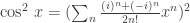
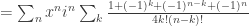
I have a somewhat different viewpoint. At the heart of the series for $\mbox{sin}$ and $\mbox{cos}$ is the periodic sequence $0,1,0,-1, 0,1\ldots$ . And surely the mathematical techniques for manipulating this series can be no simpler than the series itself! In other words, I feel that my observation that we can write this sequence as $\frac{i^n + (-i)^n}{2}$ was just notational convenience and nothing more. My own style is to prefer algebra to case analysis because I tend to make more mistakes in the latter.

To illustrate this, I am presenting the same proof, without an appeal to complex numbers. It requires a little more thought, but is overall a much simpler-looking approach.

First, for the purpose of notation, we need to make an observation about power series. If $f(x) = \sum_n \frac{a_n x^n}{n!}$ and $g(x) = \sum_n \frac{b_n x^n}{n!}$ , then $f(x)g(x) = \sum_n x^n \sum_k \frac{a_k b_{n-k}}{k! (n-k)!} = \sum_n \frac{x^n}{n!} \sum_k {n\choose k}a_k b_{n-k}$ . Nothing special here; just the distributive law. (if you are interested in going deeper into these kinds of manipulations of sequences, I highly recommend Wilf’s generatingfunctionology, available for free online)

In the same notation, if $f(x)=\mbox{sin}\ x$ and $g(x)=\mbox{cos}\ x$ , then $a_n$ and $b_n$ are the sequences $0, 1, 0, -1\ldots$ and $1,0,-1,0\ldots$ respectively.

Steps 1 and 2:

$\mbox{sin}\ x = \sum_n \frac{a_n x^n}{n!}$

$\mbox{sin}^2\ x = \sum_n \frac{c_n x^n}{n!}$

where $c_n = \sum_k {n\choose k} a_k a_{n-k}$ , and

$\mbox{cos}\ x = \sum_n \frac{b_n x^n}{n!}$

$\mbox{cos}^2\ x = \sum_n \frac{d_n x^n}{n!}$

where $d_n = \sum_k {n\choose k} b_k b_{n-k}$

Step 3:

$\mbox{sin}^2\ x + \mbox{cos}^2\ x = \sum_n \frac{x^n}{n!} e_n$

where $e_n = c_n + d_n$ .

We have $c_0 = 0$ and $d_0=1$ , so $e_0=1$ . All that remains to be shown is that $e_n=0$ for all $n>0$ .

First, suppose that $n$ is odd. Then $a_k a_{n-k} = b_k b_{n-k}=0$ for all $k$ , so $e_n = 0$ .

Now, suppose that $n=2m$ is even. Then $c_n = (-1)^{m+1}( {n\choose 1} + {n\choose 3}+\ldots + {n\choose {n-1}} )$ and $d_n = (-1)^m ({n\choose 0} + {n\choose 2}\ldots+ {n\choose n})$ . Hence $e_n = c_n + d_n = (-1)^m ({n\choose 0} - {n\choose 1} + {n\choose 2}\ldots + {n\choose n})$ $= (-1)^m (1-1)^n = 0$ .

9 Comments | Uncategorized | Permalink
Posted by lydianrain

All About (regular) n-gons—session at the Berkeley Math Circle

December 21, 2008

Last Tuesday I gave a talk at the Berkeley Math Circle titled “All About (regular) n-gons”. This was a sort of problem seminar that covered a mixed bag of mathematical tricks, but one focus was the use of complex numbers in geometry.

You can download my handout here. The questions range from fairly basic geometry to research questions—the question “How many intersection points are formed when we draw all the diagonals of a regular $n$ -gon?” is much more difficult than it appears at first; it was first answered in closed form by Poonen and Rubenstein in 1997.

There was a follow-up problem session this morning, which discussed some of the harder questions. (though I have yet to see solutions to either of the Miklós Schweitzer problems) I was impressed to see more than half a dozen students, many of them in junior high, spend two hours on Saturday morning like this.

The last time I talked at Berkeley Math Circle was in 2002, on generating functions.

Here are some of the more fun problems from my session this week:

What are all the values of $n$ for which you can tile the plane with regular $n$ -gons of varying size?
(Romania 1995) Find the number of ways of coloring the vertices of a regular $n$ -gon with $p$ colors, such that no two adjacent vertices have the same color.
Does there exist a regular $n$ -gon such that exactly half of its diagonals are parallel to one of its sides?
Show that the sum of the squares of the lengths of all sides and diagonals emanating from a vertex of a regular $n$ -gon inscribed in the unit circle is $2n$ .
(USAMO 1997) To clip a convex $n$ -gon means to choose a pair of consecutive sides $AB$ , $BC$ and to replace them with three segments $AM$ , $MN$ , $NC$ , where $M$ is the midpoint of $AB$ and $N$ is the midpoint of $BC$ . In other words, one cuts off the triangle $MBN$ to obtain a convex $(n+1)$ -gon. A regular hexagon $P_6$ of area $1$ is clipped to obtain a heptagon $P_7$ . Then $P_7$ is clipped (in one of the seven possible ways) to obtain an octagon $P_8$ and so on. Prove that no matter how the clippings are done, the area of $P_n$ is greater than $1/3$ for all $n\geq 6$ .
(USAMO 2008) Let $P$ be a convex polygon with $n$ sides, $n\geq 3$ . Any set of $n-3$ diagonals that do not intersect in the interior of a polygon determine a triangulation of $P$ into $n-2$ triangles. If $P$ is regular and there is a triangulation of $P$ consisting only of isoceles triangles, find all possible values of $n$ .

Leave a Comment » | Uncategorized | Permalink
Posted by lydianrain

The Group of Units (mod n)

November 24, 2008

The ring $\mathbb{Z}/n\mathbb{Z}$ is more interesting than it is often given credit for. This post will tell you the isomorphism type of its group of units.

Why care about such a simple thing? Well first, the rings $\mathbb{Z}/n\mathbb{Z}$ are universal, in the following sense. If $R$ is any ring with unity, there exists a unique $n\geq 0$ and injective homomorphism $f: \mathbb{Z}/n\mathbb{Z} \to R$ . $n$ here is called the characteristic of $R$ . It’s easy to find this homomorphism: there is a natural map $\mathbb{Z}\to R$ , and we factor out its kernel (which is of the form $n\mathbb{Z}$ , $\mathbb{Z}$ being a principal ideal domain). So we should expect $\mathbb{Z}/n\mathbb{Z}$ to come up anywhere that rings do (though $n=1$ only applies to a single ring, and $n=0$ is disproportionately common).

Theorem: If $n=2^l \prod_i p_i^{a_i}$ , where the product is over odd primes, the group of units $(\mathbb{Z}/n\mathbb{Z})^\times$ can be written as a product of cyclic groups $\prod_i Z_{p^i - p^{i-1}}$ when $l\leq 1$ and $Z_2 \times Z_{2^{l-2}} \times \prod_i Z_{p^i - p^{i-1}}$ when $l\geq 2$ . In particular, the group of units is cyclic exactly when $n$ is a power of an odd prime, twice a power of an odd prime, or $4$ .

The rest of this post will prove this theorem. First, the Chinese remainder theorem tells us that if $n$ factors into primes as $n=\prod_i p_i^{a_i}$ , then $\mathbb{Z}/n\mathbb{Z} \cong \prod_i \mathbb{Z}/p_i^{a_i} \mathbb{Z}$ . So we only need to address the question when $n=p^k$ is a power of a prime.

What are the invertible elements in $\mathbb{Z}/p^k \mathbb{Z}$ ? If $p\bigm| a$ , then $p^{k-1} a =0$ , so $a$ cannot be invertible. Those who are quick on the draw with the number theory will be able to quickly show that if $p$ does not divide $a$ , then $a$ is invertible in $\mathbb{Z}/p^k \mathbb{Z}$ . (the standard technique here is to note that $a$ and $p^k$ are relatively prime, so we can choose integers $x$ and $y$ such that $ax + p^k y = 1$ )

Since there are $p^{k-1}$ elements divisible by $p$ , it follows that $\mathbb{Z}/p^k\mathbb{Z}$ has $p^k-p^{k-1}$ units. (notice that this, along with the Chinese remainder theorem, gives us a nice formula for Euler’s phi function)

Proposition 1: When $p$ is odd, the group of units of $\mathbb{Z}/p^k\mathbb{Z}$ is a cyclic group of order $p^k-p^{k-1}$ .

Proof: The case $k=1$ is actually the most difficult. It is a special case of a theorem which says that a finite subgroup of the multiplicative group of any field is cyclic. For a proof of this case, see e.g. here. (I will certainly discuss this topic in detail in a future post)

Suppose that $\sigma$ is a generator for the group of units of $\mathbb{Z}/p \mathbb{Z}$ . Then the order of $\sigma\ (\rm{mod}\ p^k)$ is divisible by $p-1$ , so it is of the form $p^j (p-1)$ . Then $\sigma^{p^j}$ has order $p-1$ . We claim that $1+p$ has order $p^{k-1}$ , from which it follows that $\tau = \sigma^{p^j} (1+p)$ has order $p^{k-1} (p-1)=p^k -p^{k-1}$ .

What we really need to show here is that $(1+p)^{p^{k-2}} - 1$ is divisible by $p^{k-1}$ but not $p^k$ . But this is straightforward induction: if $(1+p)^{p^{k-2}} = 1 + a p^{k-1}$ with $a$ not divisible by $p$ , then taking $p$ -th powers we see that $(1+p)^{p^{k-1}} = 1 + ap^k + (\ldots)p^{k+1}$ .

Proposition 2: If $k\geq 3$ , the group of units of $\mathbb{Z}/2^k\mathbb{Z}$ is the product of two cyclic groups, one of order $2$ , and one of order $2^{k-2}$ . If $k\leq 2$ , the group of units of $\mathbb{Z}/2^k\mathbb{Z}$ is cyclic.

Proof In fact, we will show that $5$ generates a cyclic group of order $2^{k-2}$ that does not contain $- 1$ , an element of order $2$ . (there is nothing special about $5$ here—any choice that is $5\ (\rm{mod}\ 8)$ will work) We first show, by induction on $k$ , that $5^{2^{k-3}} \equiv 1+2^{k-1}\ (\rm{mod}\ 2^k)$ , the case $k=3$ being clear.

For $k\geq 3$ , the inductive hypothesis now tells us that $5^{2^{k-3}} \equiv 1+2^{k-1}\ (\rm{mod}\ 2^k)$ , so there is some $a\in\{0,1\}$ such that $5^{2^{k-3}} \equiv 1+2^{k-1} + a 2^k\ (\rm{mod}\ 2^{k+1})$ . Squaring, we get $5^{2^{k-2}} \equiv 1+2^k\ (\rm{mod}\ 2^{k+1})$ .

Since $1+2^{k-1}$ is an element of order $2$ , this shows that $5$ generates a cyclic group of order $2^{k-2}$ . So we just need to make sure that $-1\not\in \langle 5\rangle$ . But a cyclic group can contain at most one element of order $2$ , and we have already shown $1+2^{k-1}\in\langle 5\rangle$ .

The second statement in the proposition is easily verified.

Exercise: Prove the second sentence of the theorem! (hint: for one direction, use the Chinese remainder theorem for cyclic groups, and for the other, count elements of order $2$ )

Leave a Comment » | Uncategorized | Permalink
Posted by lydianrain

Fun With Group Actions

November 10, 2008

I had to take a bit of a break to move into my new apartment in the Castro, (which has, incidentally, been a pretty exciting place to live this past week) but now I’m all settled down and ready to tell you about group actions.

The basic idea of a group action is to visualize a group as a set of permutations of some set $X$ , giving a homomorphism $\phi: G\to S_{|X|}$ . A basic example would be the cyclic group $Z_n$ acting on an $n$ -gon by rotation. But here are some more interesting and general group actions for a group $G$ :

$G$ acts on $G$ by left multiplication.
$G$ acts on a normal subgroup of $G$ by conjugation.
$G$ acts on the set of subgroups of $G$ of a fixed order, by conjugation.
If $H\leq G$ , $G$ acts on the set of left cosets of $H$ by left multiplication.

All of these can provide useful information through the existence of homomorphisms to some symmetric group $S_n$ . For an example of this technique, let’s consider this classic problem:

Problem: Show that any simple group of order $60$ is isomorphic to $A_5$ . (recall that a simple group is one with no nontrivial normal subgroups)

We make use of some basic Sylow theory. Let $G$ be a simple group of order $60$ and let $k$ be the number of subgroups of $G$ that have order $5$ . Sylow’s theorems tell us that $k$ is a factor of $12$ and is congruent to $1\ (\rm{mod}\ 5)$ , so $k\in \{1,6\}$ . If $k=1$ , then the group of order $5$ is normal, (do you see why?) so $k=6$ .

Let $G$ act on the set of subgroups of $G$ of order $5$ , by conjugation. This gives a homomorphism $\phi: G\to S_6$ . Because none of these subgroups can be normal (or again appealing to Sylow theory) it is easy to see that $\phi\neq 1$ , so $\ker{\phi}\neq G$ . But $\ker{\phi}$ is a normal subgroup of $G$ , so $\ker{\phi}=1$ and $\phi$ is injective.

So we can imagine $G$ as a subgroup of $S_6$ . In fact, $\phi(G)\leq A_6$ , as the following lemma will tell us:

Lemma: If $H\leq S_n$ is a simple group of order larger than $2$ , $H\leq A_n$ .

Proof: Let $\sigma: S_n\to Z_2$ be the sign homomorphism, so $A_n = \ker{\sigma}$ . Then $\ker{\sigma_H}$ is a normal subgroup of $H$ . But $\sigma_H$ cannot be injective, as $|H|>|Z_2|$ , so $\ker{\sigma_H} = H$ , in other words $H\leq \ker{\sigma}=A_n$ .

Returning to our solution, we can now assume that $G\leq A_6$ . Counting orders, we see that $G$ has index $360/60=6$ . Let $A_6$ act on the set of left cosets of $G$ by left multiplication, giving a homomorphism $\psi: A_6 \to S_6$ . Pausing for a moment to verify that $\psi\neq 1$ , the fact that $A_6$ is simple tells us that $\psi$ is injective, and applying the lemma tells us easily that $\psi:A_6\to A_6$ is an isomorphism.

What is the image of $G$ under this isomorphism? Well, let’s think about the action again. We have some cosets $x_1 G, x_2 G, x_3 G, x_4 G, x_5 G, G$ . Multiplication on the left by elements of $G$ is certainly not guaranteed to fix the first five, but it will always fix the last one. In other words, $\psi(G)\leq S_5$ . So $\psi(G)\leq S_5 \cap A_6=A_5$ .

Since $|G|=|A_5|$ , it follows that $\psi$ is an isomorphism carrying $G$ to $A_5$ , and we are done.

As we can see, group actions provide an excellent if somewhat magical way of reasoning about finite groups that are too big to be easily understood by hand. Make them part of your group theory toolbox.

Leave a Comment » | Uncategorized | Permalink
Posted by lydianrain

The “Injectivity Implies Surjectivity” Trick

October 18, 2008

There is a standard proof technique involving the relationship between injectivity and surjectivity on “finite” structures. I rather like it—for the examples provided, it is very difficult to proceed without knowing the trick, even though the solutions are very simple.

Principle A: If $S$ is a finite set and $\phi: S\to S$ is a function, then $\phi$ is injective if and only if $\phi$ is surjective.

Proposition 1: If $\mathbb{F}$ is a finite field and $\phi:\mathbb{F}\to\mathbb{F}$ is a homomorphism of fields, then $\phi$ is an isomorphism.

Proof: $\ker{\phi}$ is an ideal of $\mathbb{F}$ , but it cannot equal $\mathbb{F}$ , (for $\phi(1)=1$ ) so $\ker{\phi}=0$ and $\phi$ is injective. Therefore $\phi$ is surjective.

Proposition 2: If $G$ is a finite simple group and $\phi:G\to G$ is a homomorphism, then $\phi$ is an isomorphism or $\phi\equiv e$ .

Proof: Either $\ker{\phi}=G$ , in which case $\phi\equiv e$ , or $\ker{\phi}=\{e\}$ , in which case $\phi$ is injective, so $\phi$ is surjective.

Principle B: If $V$ is a finite dimensional vector space and $\phi:V\to V$ is a linear transformation, then $\phi$ is injective if and only if $\phi$ is surjective.

Proposition 3: If $K$ is a field and $A$ is an integral domain containing $K$ with finite dimension over $K$ , then $A$ is a field.

Proof: It suffices to show that we can take inverses. Choose any nonzero $a\in A$ , and consider the map $\phi: A\to A$ defined by $\phi(x) = ax$ . Then $\phi$ is a linear transformation. Since $A$ is an integral domain, $\phi$ is injective, therefore $\phi$ is surjective. So there exists some $b\in A$ with $\phi(b)=1$ , so $ab=1$ .

Problem: Show that any finite integral domain is a field.

EDIT: As Steven points out in the comments, the following is also useful, and the proof is a good exercise:

Principle C: If $M$ is a Notherian module then any surjective homomorphism $\phi: M\to M$ is injective, and if $M$ is an Artinian module, then any injective homomorphism $\phi:M\to M$ is surjective. (hint: in fact, for any $\phi:M\to M$ , if $M$ is Noetherian, then for large enough $n$ we have $\ker{\phi^n} \cap \rm{image}\ \phi^n = 0$ . If $M$ is Artinian, then for large enough $n$ we have $\ker{\phi^n} + \rm{image}\ \phi^n = M$ .)

6 Comments | Uncategorized | Permalink
Posted by lydianrain

An Easy Fallacy

October 12, 2008

For a change of pace today, I’ll present an incorrect proof of a simple proposition. The diligent reader can work out the location of the mistake before reading on, where I will present a modified proposition, and correct proof, before discussing the mistake in detail.

Proposition: If $k$ is a field and $c$ is a cardinal less than $|k|$ , then a vector space over $k$ cannot be written as a union of $c$ of its proper subspaces.

Questionable Proof: Suppose that $\{V_\alpha\}$ is a collection of $c$ proper subspaces of $V$ , which cover $V$ . We can assume that no proper subcollection covers $V$ . (we can remove the superfluous elements from our collection if this is not the case) This implies that for each $\alpha$ , there exists some $v_\alpha \in V_\alpha$ such that $v_\alpha \not\in V_\beta$ for $\beta\neq\alpha$ .

Take any $\alpha\neq\beta$ , and consider the set $\{v_\alpha + \lambda v_\beta\ |\ \lambda \in k\}$ . This set has cardinality $k$ , and each element lies in some $V_\gamma$ , so by the pigeonhole principle, two of these elements must lie in the same $V_\gamma$ , say $v_\alpha + \lambda_1 v_\beta \in V_\gamma$ and $v_\alpha + \lambda_2 v_\beta \in V_\gamma$ .

Subtracting, we see that $(\lambda_1 - \lambda_2)v_\beta \in V_\gamma$ , so $v_\beta \in V_\gamma$ . Therefore $\beta = \gamma$ . Similarly, we see that $v_\alpha\in V_\gamma$ , so $\alpha=\gamma=\beta$ , contradiction.

The above proposition is, unfortunately, false. To see this, take $V$ to be a real vector space with countably infinite basis $e_1,e_2,\ldots$ , and for each $i$ , let $V_i$ be the vector space generated by $e_j$ , $j\neq i$ . Then $\{V_i\}$ covers $V$ , even though it is a set of cardinality $\aleph_0 < |\mathbb{R}|$ .

We need to add a condition to the proposition, but this time the proof is correct.

Modified Proposition: If $k$ is a field and $c$ is a cardinal less than $|k|$ , then a finite dimensional vector space over $k$ cannot be written as a union of $c$ of its proper subspaces.

Proof: We proceed by induction on the dimension. If $V$ has dimension $1$ , then any union of proper subspaces must be the zero space, so the statement is trivial. Now assume that $V$ has dimension $d \geq 2$ and the proposition has been proved for all vector spaces of dimension $d-1$ .

First, observe that there are at least $|k|$ subspaces of $V$ of dimension $d-1$ . For if $e_1,\ldots e_n$ are a basis for $V$ , then we can take the subspaces generated by $\lambda e_1 + e_2, e_3,\ldots e_n$ for $\lambda\in K$ .

Suppose that we are given a collection $\{V_\alpha\}$ of proper subspaces of $V$ of cardinality $c$ that covers $V$ . Since there are at least $|k|> c$ spaces of dimension $d-1$ , there must be such a space $W$ that is not equal to any $V_\alpha$ . Hence $\{V_\alpha \cap W\}$ is a collection of proper subspaces of $W$ of cardinality $c$ that covers $W$ , contradiction.

So what was the mistake in the original proof? You might question my use of the pigeonhole principle on infinite sets, but that can actually be made quite rigorous. No, the problem is the statement “We can assume that no proper subcollection covers $V$ “. Though an attractive idea, it is not true that we can reduce our collection to no longer be redundant.

Consider our earlier counterexample, a real vector space with a countably infinite basis. The given collection covers $V$ , but there is no non-redundant subcollection that does so. A slightly painful reminder that we must always modify our intuition when dealing with infinite sets.

We can salvage the original proof, however, when the collection is finite. Then, in fact, we can throw out elements of our collection, one at a time, until we have eliminated any redundancy. That gives us the following: (note that this is not strictly weaker than our modified proposition, since it applies to infinite-dimensional spaces as well)

Salvaged Proposition: If $k$ is an infinite field, a vector space over $k$ cannot be written as a union of finitely many proper subspaces.

1 Comment | Uncategorized | Permalink
Posted by lydianrain

Geometric Complex Analysis: Rouché’s Theorem

October 3, 2008

Complex analysis is one of the most rich and amazing areas of mathematics, for the complex numbers $\mathbb{C}$ possess geometric properties that intertwine with their analytic properties in surprising and beautiful ways. This is hardly a place to discuss the subject in detail, so I will focus on Rouché’s Theorem, with an entertaining application.

Rouché’s Theorem If $U$ is an open disc in $\mathbb{C}$ , and $f$ and $g$ are complex-valued differentiable functions defined in some neighborhood of $\overline{U}$ , and if $|f+g| < |g|$ on the boundary of $U$ , then $f$ and $g$ have the same number of zeros inside $U$ , up to multiplicity.

By “multiplicity” here we mean the following: $\alpha$ is a zero of multiplicity 1 of $h$ if $h(\alpha)=0$ but $h'(\alpha)\neq 0$ , and a zero of multiplicity two if $h(\alpha)=h'(\alpha)=0$ but $h''(\alpha)\neq 0$ , etc.

The Wikipedia article on this theorem has an interesting informal summary: “If a person were to walk a dog on a leash around and around a tree, and the length of the leash is less than the radius of the tree, then the person and the dog go around the tree an equal number of times.” A little bit of an oversimplification perhaps, but an alluring hint at the deep geometric principles at work in this theorem.

An application:

Proposition: For any $n=2,3,\ldots$ , the polynomial $p_n(x) = 1 - x - x^2 - \ldots - x^n$ is irreducible.

Proof: Let $f(x) = (1-x)p_n(x) = x^{n+1} - 2x + 1$ , and let $g(x) = 2x$ . Choose $r < 1$ to be sufficiently close to $1$ that $r^{n+1}+1 < 2r$ .

Then, when $|x| = r$ , we have $|f(x) + g(x)| = |x^{n+1} + 1| \leq r^{n+1} + 1 \leq 2r = |2x| = |g(x)|$ , so $f$ and $g$ satisfy the conditions of Rouché’s Theorem, and have the same number of zeros inside the circle around the origin of radius $r$ . Letting $r\to 1^-$ , we find that $f$ and $g$ have the same number of roots inside the circle of radius $1$ .

But $g$ has exactly one root inside this circle, so $f$ , hence $p_n(x)$ must have exactly one root $\alpha$ with $|\alpha| < 1$ .

Now, suppose that $\beta$ were a root of $f(x)$ with $|\beta| = 1$ . Then $\beta - 1/2 = \beta^{n+1}/2$ , so $|\beta - 1/2| = 1/2$ . So $\beta$ lies on a circle around $1/2$ of radius $1/2$ , as well as on the circle around the origin of radius $1$ , so $\beta=1$ . Since $p_n(1) = 1-n\neq 0$ , $p_n(x)$ has no roots on the unit circle.

Now we are done! For if $p_n(x) = a(x)b(x)$ over the integers, then the constant terms of $a$ and $b$ must be $\pm 1$ . But these constant terms are the product of some subset of the roots of $p_n$ . If $\alpha$ is a root of $a$ , since it is the only root of absolute value less than or equal to one, it follows that $a$ must have every single other root of $p_n$ as a root, and the factorization must be trivial.

For anyone interested in studying this subject in greater detail, I highly recommend Functions of One Complex Variable by John B. Conway. And if you want to know more about numbers like our $\alpha$ above, read up on Pisot numbers.

1 Comment | Uncategorized | Permalink
Posted by lydianrain

What’s The Deal With Hausdorff Spaces? (Part II)

September 22, 2008

Last time, we learned that—in a world in which much is uncertain—at least we can trust continuous maps of Hausdorff spaces to behave nicely with respect to dense subsets.

Or can we? We showed that if $S\subset X$ is dense, then any continuous map $f: X\to Y$ is determined by its values on $S$ , which jives well with our intuition about maps $f :\mathbb{R}\to\mathbb{R}$ , for example.

But in $\mathbb{R}$ we can go ever farther. For any open set $U\subset\mathbb{R}$ , we can construct a bump function that is nonzero on $U$ , but zero outside of $U$ . It follows that if $S\in\mathbb{R}$ is not dense, then continuous functions $f:\mathbb{R}\to\mathbb{R}$ are not determined by their values on $S$ .

Is this true of all Hausdorff spaces?

The answer is yes, but proving it requires some creativity. The brute force approach does not work here—there is no clear way to create a bump function on some arbitrary space. If you consider yourself a point-set topology guru, I encourage you to try to prove the proposition yourself before reading on.

Proposition: If $X$ is a Hausdorff space and $S\subset X$ is not dense, then there exists some Hausdorff space $Y$ and two distinct continuous functions $f,g: X\to Y$ that agree on $S$ .

Proof: Let $K=\overline{S}$ , and let $Y$ be two copies of $X$ glued together along $K$ . Since there are points not in $K$ , the two embeddings $f,g:X\to Y$ are distinct, but agree on $K$ by construction.

I have kept the proof (extremely) short to illustrate the beauty of the idea, but there are a few assumptions that need to be justified. The most serious of these is the assertion that $Y$ is Hausdorff. But a little reading on disjoint unions and quotient spaces will reveal that this is not particularly difficult. (though it is very necessary to know that $K$ is closed)

I do not know if this result is as strong as possible. So I leave the question to you, if you hunger and thirst for more than these two articles have provided.

Question: Does there exist some $T_1$ space $X$ and a non-dense subset $S\subset X$ such that any continuous map $f:X\to Y$ , where $Y$ is Hausdorff, is determined by its values on $S$ ?

Leave a Comment » | Uncategorized | Permalink
Posted by lydianrain

What’s The Deal With Hausdorff Spaces? (Part I)

September 14, 2008

If you have spent more than a few minutes with point-set topology, chances are that you have heard the term “Hausdorff space.” The axioms of a topological space are perhaps a little too general, and so most topological theorems impose additional axioms. Here are some of the basic separation axioms:

A space is called $T_0$ if for any two distinct points $x$ and $y$ , there exists an open set $U$ that contains exactly one of $x$ and $y$ .

A space is called $T_1$ if for any two distinct points $x$ and $y$ , there exists an open set $U$ that contains $x$ but not $y$ , and an open set $V$ that contains $y$ but not $x$ .

A space is called $T_2$ , or Hausdorff, if for any two distinct points $x$ and $y$ , there exist disjoint open sets $U$ and $V$ such that $U$ contains $x$ and $V$ contains $y$ .

It should be clear that Hausdorff spaces are $T_1$ , and $T_1$ spaces are $T_0$ . One example of a $T_1$ space that is not Hausdorff is the integers, where $U\subset \mathbb{Z}$ is an open set if $\mathbb{Z}-U$ is finite.

There are many, many other separation axioms, in fact, there are increasingly strong axioms called $T_3$ , $T_4$ , $T_5$ , and $T_6$ . So why is the Hausdorff axiom so important?

One possible explanation involves dense sets. If $X$ is a topological space, a set $S\in X$ is called dense if every nonempty open set $U\subset X$ contains a point from $S$ . For example, $\mathbb{Q}\subset\mathbb{R}$ is dense. Notice that any continuous function $f: \mathbb{R}\to \mathbb{R}$ is determined entirely by its values on $\mathbb{Q}$ . This can be generalized:

Proposition: If $X$ is a topological space, $S\subset X$ is dense, and $Y$ is a Hausdorff space, then any continuous function $f: X\to Y$ is determined by its values on $S$ .

Proof: We show that two functions that are equal on $S$ are equal everywhere. Suppose that $f, g: X\to Y$ are continuous and not equal. Then $\exists x\in X$ such that $f(x)\neq g(x)$ .

By the Hausdorff condition, we can choose disjoint open sets $U$ and $V$ with $f(x)\in U$ and $g(x)\in V$ . Then $f^{-1} (U)\cap f^{-1}(V)$ is a nonempty open set in $X$ , so it contains a point $s\in S$ . Hence $f(s)\in U$ and $g(s)\in V$ , so $f(s)\neq g(s)$ , and $f\neq g$ on $S$ .

Furthermore, there exist $T_1$ spaces $Y$ for which the above proposition fails. In fact, our above example is one case: the space $X=\mathbb{Z}$ with the cofinite topology.

$X$ is $T_1$ , which is not so hard to verify. It is also not hard to verify that if $S\subset \mathbb{Z}$ is infinite, then $S$ is dense.

Also, any bijective function $f: X\to X$ is continuous. But a bijection cannot be determined by its value on all but two points, so if we choose $S$ so that $X-S$ contains at least two points, then continuous functions $X\to X$ are not determined by their value on $S$ .

I feel that this example gives some insight into why Hausdorff spaces are studied so frequently, or at least why they are “just nice enough” in many circumstances.

And next week, I’ll post an exciting converse to the proposition.

1 Comment | Uncategorized | Permalink
Posted by lydianrain

Archives